NIM: 2301884803
Name: Erdvin
Selasa, 9 Juni 2020
Class: CB01
Lecturer: Henry Chong (D4460) and Ferdinand Ariandy Luwinda (D4522)
Introduction to Linked List
----------------------------------------------------------------------
Linked List is one of the many types of Data Structure. In a Linked List, each data record is accompanied with a reference to the next data record, and in certain variations, a reference to the previous data record. A Linked List has the advantage of being able to insert and delete any data record from any location. This makes a Linked List suitable for real-time programs where the amount of data is hard to predict and for programs that require accessing the data records sequentially. However, Linked Lists makes it hard to search for a specific data, as it doesn't allow for random access and has to check each data one-by-one sequentially. It also takes up a large amount of memory.
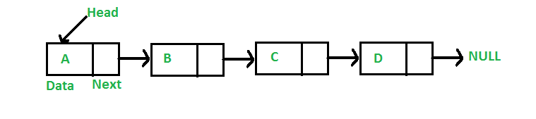
A Linked List are based around the usage of 'Nodes', which contains a data record and an address pointing to the next node. Some Linked Lists also have an additional address, pointing to the previous node. To determine which Node the program will add a data record to, Linked Lists makes use of a 'Head' address. The Head address usually begins at the first Node before moving to other Nodes. At the end of a Linked List is a 'Null' address to indicate that the Linked List has ended.
Types of Linked List
----------------------------------------------------------------------
Linked Lists have multiple variations, the most popular of them include:
- Singly Linked List
Singly Linked List is the most basic form of a Linked List, and contains only the minimum of what a Linked List has. Within the node, there only exists an address to the next node.
This is how a Singly Linked List node looks like in C:
struct Node {
int data;
struct Node* next;
};
Visual example of a Singly Linked List:
- Circular Linked List
Circular Linked List is virtually the same as with a Singly Linked List, but at the end of the Linked List, the Null address is replaced by an address that points to the first Node. This type of Linked List can be used if the program has to cycle through the List multiple times.
Visual example of a Circular Linked List:
- Doubly Linked List
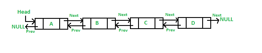
In a Doubly Linked List, the Node does not only contain an address for the next Node, but also an address pointing to the previous Node. This makes it faster to insert and delete Nodes that are located in the middle, but also uses more memory than a Singly Linked List.
This is how a Doubly Linked List node looks like in C:
struct Node {
int data;
struct Node* next; // Pointer to next node in DLL
struct Node* prev; // Pointer to previous node in DLL
};
Visual example of a Doubly Linked List:
- Circular Doubly Linked List
Circular Doubly Linked List combines the features of Circular and Doubly Linked List along with the inherent advantages that comes with it, but has the obvious drawback of taking up more memory.
Visual example of a Doubly Linked List:
Insertion and Deletion
----------------------------------------------------------------------
One of the main advantages that a Linked List has to offer is that it can insert and delete Nodes from any location. To better explain this advantage point, we will look at snippets of how insertion and deletion can be done in Singly Linked Lists. These snippets are taken from geeksforgeeks.org
In Linked Lists, insertion is done by allocating the memory for a new Node, putting in the data into the Node and then placing the Node in the required position. Linked List insertion has three main variants, insertion from the front, in the middle, and at the end of the List.
We will begin with insertion from the front. In C, this would look like:
void push(struct Node** head_ref, int new_data)
{
/* 1. allocate node */
struct Node* new_node = (struct Node*) malloc(sizeof(struct Node));
/* 2. put in the data */
new_node->data = new_data;
/* 3. Make next of new node as head */
new_node->next = (*head_ref);
/* 4. move the head to point to the new node */
(*head_ref) = new_node;
}
Now, let us compare with insertion in the middle of the Linked List and at the end of the Linked List. In C, inserting between two Nodes would look like:
void insertAfter(struct Node* prev_node, int new_data)
{
/*1. check if the given prev_node is NULL */
if (prev_node == NULL)
{
printf("the given previous node cannot be NULL");
return;
}
/* 2. allocate new node */
struct Node* new_node =(struct Node*) malloc(sizeof(struct Node));
/* 3. put in the data */
new_node->data = new_data;
/* 4. Make next of new node as next of prev_node */
new_node->next = prev_node->next;
/* 5. move the next of prev_node as new_node */
prev_node->next = new_node;
}
The main difference between the two is that when inserting in the middle, the program has to check whether the query given for where the new Node would be is Null or not. Other than that, these two are the same.
As for insertion at the end of the List, in C it would look like:
void append(struct Node** head_ref, int new_data)
{
/* 1. allocate node */
struct Node* new_node = (struct Node*) malloc(sizeof(struct Node));
struct Node *last = *head_ref; /* used in step 5*/
/* 2. put in the data */
new_node->data = new_data;
/* 3. This new node is going to be the last node, so make next
of it as NULL*/
new_node->next = NULL;
/* 4. If the Linked List is empty, then make the new node as head */
if (*head_ref == NULL)
{
*head_ref = new_node;
return;
}
/* 5. Else traverse till the last node */
while (last->next != NULL)
last = last->next;
/* 6. Change the next of last node */
last->next = new_node;
return;
}
There are a few differences between inserting from the front and at the end. The first is that instead of pointing to the next Node, it instead points at Null. The second is that it has to first search for the last Node before inserting. Step 4 is only there to prevent an error; if this function is used anytime after using the push function, it is not required.
Linked List deletion is done by first searching for the Node that it will delete, unlink the Node and finally free the memory allocation. As for deletion, there are two variations; deleting a Node by its value or by the Node's position. In C, this code can be used to delete a Node by a key value
void deleteNode(struct Node **head_ref, int key)
{
// Store head node
struct Node* temp = *head_ref, *prev;
// If head node itself holds the key to be deleted
if (temp != NULL && temp->data == key)
{
*head_ref = temp->next; // Changed head
free(temp); // free old head
return;
}
// Search for the key to be deleted, keep track of the
// previous node as we need to change 'prev->next'
while (temp != NULL && temp->data != key)
{
prev = temp;
temp = temp->next;
}
// If key was not present in linked list
if (temp == NULL) return;
// Unlink the node from linked list
prev->next = temp->next;
free(temp); // Free memory
}
In comparison, here is what deleting by a Node's position looks like in C:
void deleteNode(struct Node **head_ref, int position)
{
// If linked list is empty
if (*head_ref == NULL)
return;
// Store head node
struct Node* temp = *head_ref;
// If head needs to be removed
if (position == 0)
{
*head_ref = temp->next; // Change head
free(temp); // free old head
return;
}
// Find previous node of the node to be deleted
for (int i=0; temp!=NULL && i<position-1; i++)
temp = temp->next;
// If position is more than number of ndoes
if (temp == NULL || temp->next == NULL)
return;
// Node temp->next is the node to be deleted
// Store pointer to the next of node to be deleted
struct Node *next = temp->next->next;
// Unlink the node from linked list
free(temp->next); // Free memory
temp->next = next; // Unlink the deleted node from list
}
As can be seen, there are not many differences between the two. The biggest difference is in what the code is searching for; a key value or a specific Node.
----------------------------------------------------------------------------------------------------------------------------------------------------------------------------------------------------------------------------------------------------------------------------------------------------------------------------------------------------
Introduction to Hash Table
----------------------------------------------------------------------
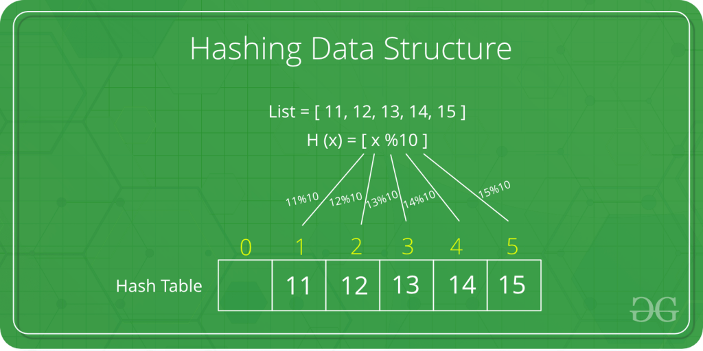
Hashing is a part of Data Structure that maps certain values with keys. These keys are shorter and easier to read than the value itself, so it is used to increase efficiency when referring to a value. How much more efficient it becomes will depend on the type of hashing that is used. A Hash Table is an array where the hash keys are stored. The method used to create the Hash Table is called Hash Function.
Example of Hash Table:
Wherein List contains the original values, H(x) is the Hash Function, and the array addresses are the keys.
Hash Functions
----------------------------------------------------------------------
There are a very wide variety of Hash Functions, but on this article, I will only explain about Mid-square, Division, Folding, Digit Extraction and Rotating Hash.
Mid-square is a Hash Function where the value is squared, and then taking the middle part of the squared value as the key. For example, with a value of 2175, it will be squared to become 4730625. We take the middle part, which is 306, to become the key. In Mid-square, collision has a low probability of occurring, but still noticeable. An example is for values 2000 and 9000, both will result in a key of 000. It is also important to remember that squaring a value may cause overflow. If an overflow occurs, it can be fixed by using long long integer data type or using string as multiplication.
Division (or also known as Mod method) is a Hash Function where the key is Value % (modulus) Constant. For example, with a value of 64971 % 97, it will result in a key of 78. It is known that Division works best with a prime number as its modulus constant. The larger the prime number, the better. Collision can still occur with any constant, for example 472819 and 740166 has the same key value, being 38.
Folding is a Hash Function where the value is partitioned, then the parts are added to form the key. For example, with a value of 56143, the value is split into 56, 14 and 3, then added to become 73. Folding is relatively fast, and also prevents Collision quite well, but not completely. For example, 12356 and 48301 both has a key of 71.
Digit Extraction is a Hash Function where digits of the value is taken to create a shorter value as the key. For example, with a value of 3728192, we take the first, third, fifth and seventh value to form 3212 as the key. Collision can occur if the digits taken are the same. For example, the values 12345 and 18355 would have the same keys.
Rotating Hash is a Hash Function where a key from another Hash Function has its rightmost digit shifted onto the leftmost digit. For example, a key of 473 becomes 347 after Rotating Hash. Rotating hash helps with preventing Collisions.
Collision Handling
----------------------------------------------------------------------
In Hashing, there is a very real possibility that Hash Functions has certain values with the same keys. This is called Collision. There are two ways to handle a collision, those being Chaining and Open Addressing.
Chaining makes use of Linked Lists so that when a Collision occurs, the key for that value will be stored in the next node. This has the disadvantage of using larger amounts of memory, and is more suitable for larger programs.
Open Addressing or Linear Probing is when a Collision occurs, the key for a certain value will change by a certain amount, such as +1, until a Collision no longer occurs. This has the disadvantage of potentially making the Hash Table hard to read.
Introduction to Tree
----------------------------------------------------------------------
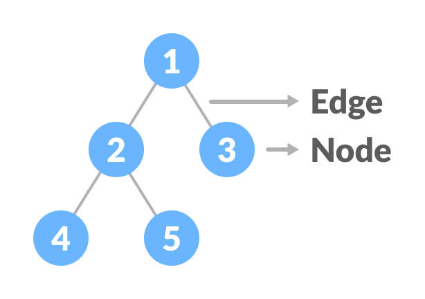
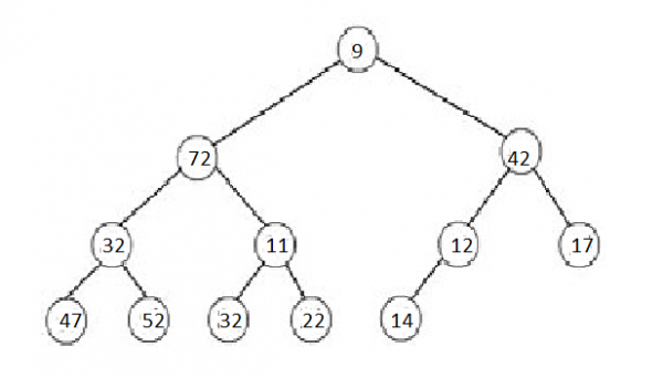
A Tree is a hierarchial Data Structure, which allows for faster and easier access. There are a number of terminologies that are used for Trees, the most basic of them being Node and Edge. Values are contained by Nodes and Nodes are connected by Edges. Here is an example of a Tree:
Other than those, Root describes the topmost Node of a Tree, a Child is a Node that branches from another Node, a Leaf is a Node that doesn't have any child and a Forest is a set of disjointed trees. A Node has Height/Depth and Degree. Height/Depth describes the number of edges towards/from the deepest leaf. The Height/Depth for a Root Node is also the Height/Depth for the Tree. Degree describes the number of branches in the Node.
Binary Tree
----------------------------------------------------------------------
Binary Tree is a Tree where each Node has a maximum of two Children. Each Node contains a data, a left pointer and a right pointer. In C, it would look like this:
struct node {
int data;
struct node *left;
struct node *right;
};
In a Binary Tree, it is possible to count the maximum possible amount of Nodes at the level "l" with the formula 2l-1 and the maximum possible amount of Nodes at height "h" with 2h – 1.
Types of Binary Trees
----------------------------------------------------------------------
Binary Trees have multiple variations, the most common of them being Perfect, Complete, Skewed and Balanced Binary Trees.
Perfect Binary Tree or Full Binary Tree is a Binary Tree where every node except for the leaves has two children. In a Perfect Binary Tree, you can count the amount of leaves by adding the number of Nodes before it + 1.
Complete Binary Tree is a Binary Tree where every level of the tree, except for maybe the last level, has the maximum amount of Nodes. A Perfect Binary Tree is always also a Complete Binary Tree.
Skewed Binary Tree or Degenerate Binary Tree is a Binary Tree where every Node has at maximum one child.
Balanced Binary Tree is a Binary Tree where none of the leaves are shorter or further than any other leaves from the root.
Expression Tree is a Binary Tree where every leaf contains an operand and every other node contains an operator. Expression Trees can be used for Prefix, Postfix and Infix Traversals.
Threaded Binary Tree is a Binary Tree variant where Node pointers previously pointing towards NULL, now points to a previous Node.
----------------------------------------------------------------------------------------------------------------------------------------------------------------------------------------------------------------------------------------------------------------------------------------------------------------------------------------------------
Introduction to Binary Search Tree
----------------------------------------------------------------------
A Binary Search Tree is a Data Structure, being a variation of Binary Tree. It is essentially a sorted version of Binary Tree, and some people refer to it as such. A Binary Search Tree has these following properties;
- The left subtree of a node contains only nodes with keys lesser than the node’s key.
- The right subtree of a node contains only nodes with keys greater than the node’s key.
- The left and right subtree each must also be a binary search tree.
A Binary Search Tree has a search time of 0(log(n)). A Binary Search Tree has the advantages of having quick searching, insertion and deletion due to being sorted.
Example of a Binary Search Tree:
If you notice, every left subtree has a smaller value compared to its parent, and every right subtree has a larger value compared to its parent.
Search Operation
----------------------------------------------------------------------
When performing a Search in Binary Search Tree, the program will first check the root value and then go from there until it finds the key value. If the key value smaller than the root or parent value, it will check the left-hand side, and if it's larger than the root or parent value, it will check the right-hand side.
Example of a Binary Search Tree Searching function in C:
struct node* search(struct node* root, int key)
{
// Base Cases: root is null or key is present at root
if (root == NULL || root->key == key)
return root;
// Key is greater than root's key
if (root->key < key)
return search(root->right, key);
// Key is smaller than root's key
return search(root->left, key);
}
The function employs simple recursion applications to perform the search.
Insertion Operation
----------------------------------------------------------------------
To perform an insertion in Binary Search Tree, the program will first check whether the tree is empty or not. If it's empty, then the current key value will become the root of the tree. If it's not empty, the program will keep checking either left for values smaller than the parent node, or right for values larger than the parent node until it finds an empty node.
Example of a Binary Search Tree Insert function in C:
struct node* insert(struct node* node, int key)
{
/* If the tree is empty, return a new node */
if (node == NULL) return newNode(key);
/* Otherwise, recur down the tree */
if (key < node->key)
node->left = insert(node->left, key);
else if (key > node->key)
node->right = insert(node->right, key);
/* return the (unchanged) node pointer */
return node;
}
The function first looks whether the current node is empty or not. If it's empty, the function ends there and the key will be inserted in that node. Otherwise, it will do a recursion in a similar fashion to the Search function until it finds an empty node.
Deletion Operation
----------------------------------------------------------------------
To perform a deletion in Binary Search Tree, the program will first check whether the root has any value or not. If it doesn't, then the function will end without doing anything. Otherwise, the function will check whether the key value is smaller, larger or is contained within the node, starting from the root.
Once the function has successfully found the node that is going to be deleted, the function performs a selection to determine how many child the node has. If the function finds it to either have no child or only one child, the function will move the other node (or if the other node is also NULL, do nothing) to the selected node. If the node does have two children, it will find the 'inorder successor', a node with the smallest value from its right-hand side. After that, it will copy the inorder successor to the selected node, then delete the node that used to house the inorder successor.
Example of a Binary Search Tree Delete function in C:
struct node* deleteNode(struct node* root, int key)
{
// base case
if (root == NULL) return root;
// If the key to be deleted is smaller than the root's key,
// then it lies in left subtree
if (key < root->key)
root->left = deleteNode(root->left, key);
// If the key to be deleted is greater than the root's key,
// then it lies in right subtree
else if (key > root->key)
root->right = deleteNode(root->right, key);
// if key is same as root's key, then This is the node
// to be deleted
else
{
// node with only one child or no child
if (root->left == NULL)
{
struct node *temp = root->right;
free(root);
return temp;
}
else if (root->right == NULL)
{
struct node *temp = root->left;
free(root);
return temp;
}
// node with two children: Get the inorder successor (smallest
// in the right subtree)
struct node* temp = minValueNode(root->right);
// Copy the inorder successor's content to this node
root->key = temp->key;
// Delete the inorder successor
root->right = deleteNode(root->right, temp->key);
}
return root;
}
This function is fairly complex until you analyze and break down what the function does. I recommend looking at the code and explanation at the same time.
----------------------------------------------------------------------------------------------------------------------------------------------------------------------------------------------------------------------------------------------------------------------------------------------------------------------------------------------------
Introduction to AVL Tree
----------------------------------------------------------------------
AVL Tree is a variation of Binary Search Tree that performs self-balancing so that the height difference between the right and left subtrees is no more than one. The advantage of having a balanced Binary Tree is having a better worst-case search speed compared to a regular Binary Search Tree. AVL Tree guarantees that the search speed will always be at O(log n).
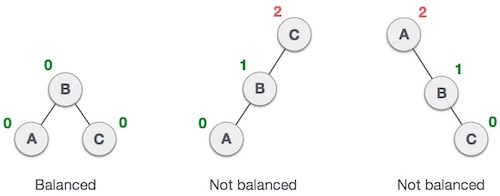
Example of what constitutes as an AVL Tree, and what doesn't:
In AVL Trees, Balance Factor refers to the height difference between the right and left subtrees. An AVL Tree may have a Balance Factor of 1, -1, or 0 to be acknowledged as an AVL Tree.
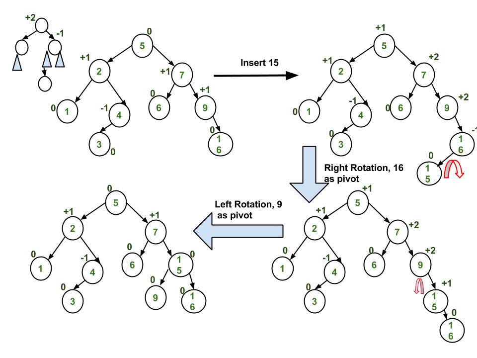
Insertion
----------------------------------------------------------------------
AVL Trees has an insertion operation like normal Binary Search Trees. However, AVL Tree checks whether the balance factor of the tree is 1, -1, or 0. If not, then it will perform rebalancing. There are four main ways to rebalance a tree, known as Left Rotation, Right Rotation, Left-Right Rotation, or Right-Left Rotation.
Insertion - Single Rotation
----------------------------------------------------------------------
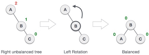
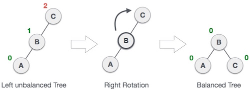
Single Rotation is a term that refers to Left Rotation and Right Rotation. It means that rebalancing the tree will only take one rotation. Left Rotation is used when the imbalance is in the left subtree, and Right Rotation is used when the imbalance is in the right subtree. Single Rotation is performed when the opposing subtree follows a straight path (left-left or right-right)
Examples of Left and Right Rotation:
Insertion - Double Rotation
----------------------------------------------------------------------
Double Rotation is a term that refers to Left-Right Rotation and Right-Left Rotation. Double Rotation is performed when the imbalance requires two rotations to be fixed. Double Rotation is performed when the opposing subtree has a zig-zag shaped path (left-right path or right-left path).
Left-Right Rotation occurs when the problem is in the right subtree of the left subtree, like so:
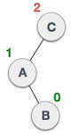
(From C, it goes a left->right path towards B)
On the other hand, Right-Left Rotation occurs when the problem is in the left subtree of the right subtree, like so:
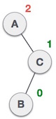
(From A, it goes a right->left path towards B)
A Double Rotation problem can be visualized as such:
What happens in both cases is that single rotation occurs two times on the "pivot".
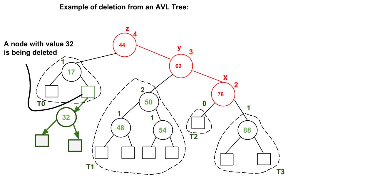
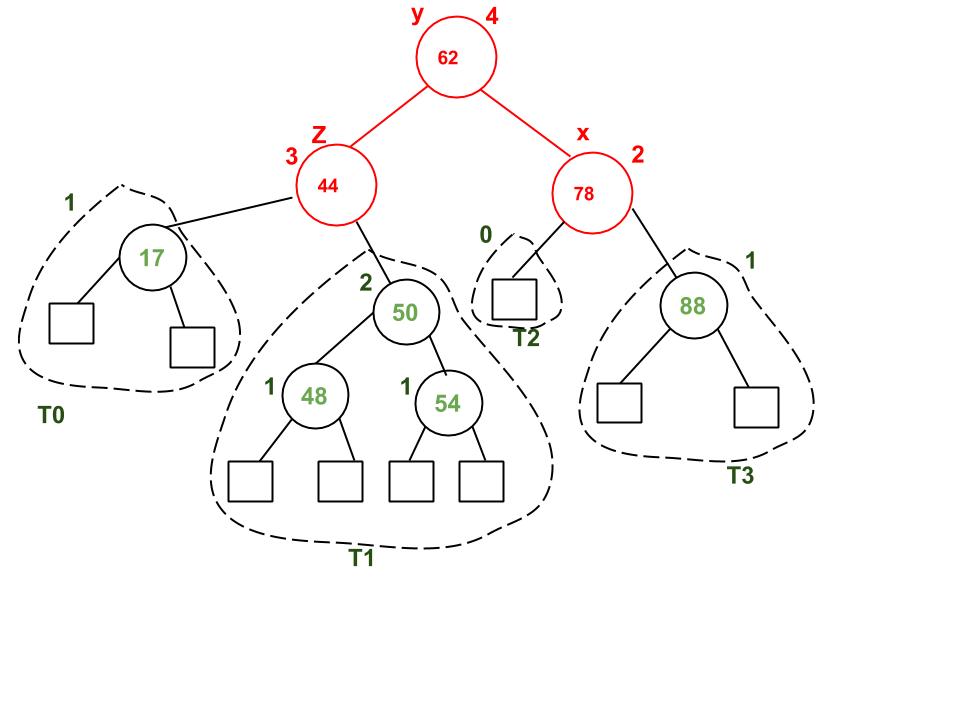
Deletion
----------------------------------------------------------------------
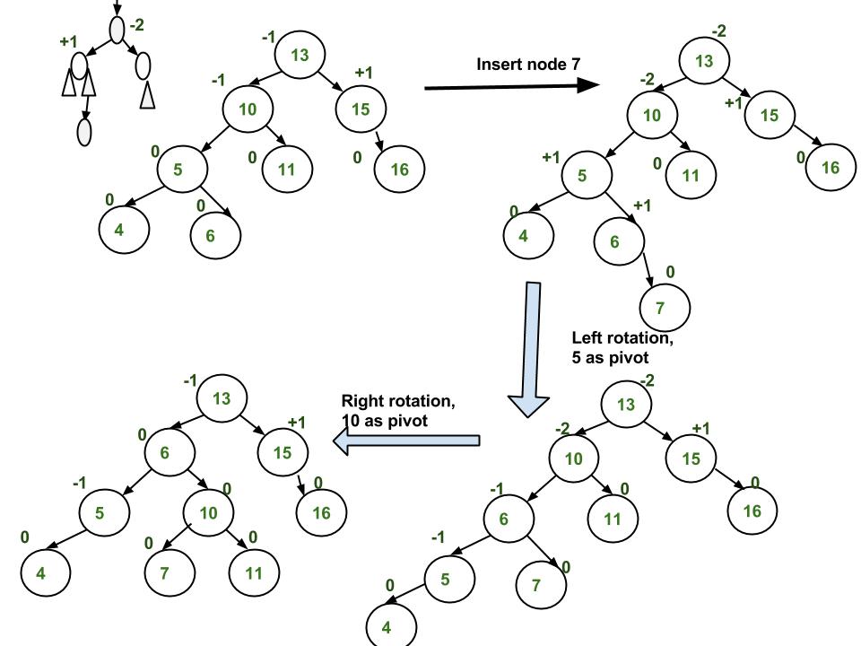
Like with Insertion, Deletion in AVL Tree is just like Deletion in a regular Binary Search Tree, and then it checks if the tree has any imbalance on it. If the balance factor after deleting a node is not 1, -1 or 0, then it will perform one of the four rotations. The main difference with AVL Tree Insertion is that after performing a rotation, it will continue to check whether an imbalance has occured on the ancestors of the rotated node.
Example of AVL Tree Deletion:
----------------------------------------------------------------------------------------------------------------------------------------------------------------------------------------------------------------------------------------------------------------------------------------------------------------------------------------------------
Introduction to Heaps
----------------------------------------------------------------------
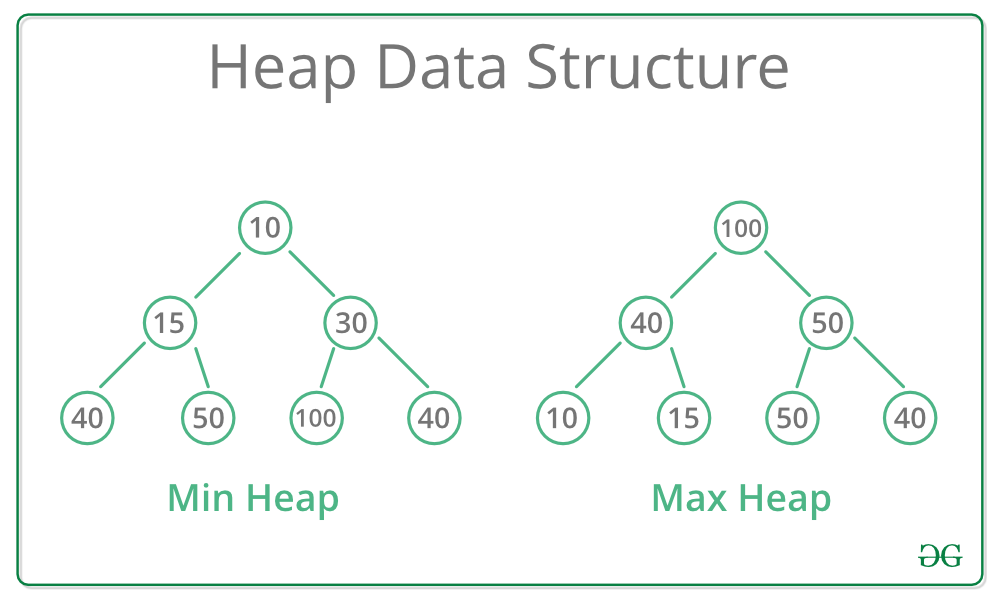
A Heap is a type of tree-based Data Structure where the Heap is always a Complete Binary Tree. Heaps are commonly used to perform Heapsort or to create Priority Queues and Graph algorithms. Heaps also have a time complexity of O(n).
Heaps are often implemented in two types; Min-Heap and Max-Heap. A Min-Heap is when the root node, or parent node during recursion, has the minimum key value for all the keys at all of its children. Max-Heap is when the root or parent node has the maximum key value instead of minimum.
Example of a Min-Heap and Max-Heap:
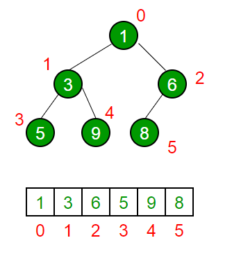
A Heap is often implemented using Arrays. The root node will always be at Arr[0], while non-root parent nodes is located at Arr[(i-1)/2]. The left child node is located at Arr[(i*2)+1], while the right child node is located at Arr[(i*2)+2]. The traversal method used in array implementation is level order.
Visual example of Heap (Min-Heap) Implementation using Arrays:
Operations on Heaps
----------------------------------------------------------------------
Heaps have a number of functions to use. The most basic of them include:
- getMin(); or getMax(); to return the root value of a Min-Heap or Max-Heap.
- Upheap refers to the process of comparing a key node with its parent node. If the key node is smaller (Min-Heap) or larger (Max-Heap) than the parent node, then the two nodes will switch places to fit with the rules of a Min-Heap or Max-Heap.
- Downheap refers to the process of comparing a key node with its children. If the key node is larger (Min-Heap) or smaller (Max-Heap) than one of its two children, then the key node and the child node will switch places.
- insert(); in Heap is done by adding the key at the end of the tree, then performing upheap recursively to ensure that the tree doesn't have any new violation.
- delete(); in Heap is used to remove the a key from Heap. The deleted node is then replaced with the last node of the tree, and the root performs downheap recursively to ensure that the tree doesn't have any new violation.
Min-Max Heap
----------------------------------------------------------------------
A Min-Max Heap is a Heap where each level alternates between Min-Heap and Max-Heap rules. Min-Levels are located at even levels (Height of 0, 2, 4, etc) while Max-Levels are located at odd levels (Height of 1, 3, 5, etc).
Visual example of a Min-Max Heap:
The root on a Min-Max Heap will have the minimum value of all its nodes. On Min-Levels, the nodes will have the smallest value among its children, while on Max-Levels, the nodes will have the largest value among its children.
A Max-Min Heap is defined as opposite to Min-Max Heap, where the root contains the maximum value in the Heap, and Min-Levels now located at odd levels while Max-Levels are now located at even levels.
Introduction to Tries
----------------------------------------------------------------------
Trie is a tree-like Data Structure where the nodes store letters of the alphabet. With Trie, words and strings can be retrieved by traversing down a Trie. The word "Trie" itself comes from "Re
Trieval". Examples of Tries Application are word prediction and spell checkers. Tries are known to have short search time, but relatively large memory usage. Trie is also known as a "Prefix Tree".
The root node of a Trie is always empty, and every node in Tries has an "End of Word" variable, usually in boolean or integer, to determine whether the node is the final letter in the word or string. Tries are implemented in a way not too different from Linked Lists.
Example of a Trie:
Tries - Insertion
----------------------------------------------------------------------
In Trie, the insertion key is a word, and insertion works by checking whether or not the prefix of the key already exists or not. If it doesn't exist, then it creates a new node from the current line of prefixes. If the key already exists from the prefixes from another word, then the program simply changes the "End of Word" variable to "True".
For example, imagine an empty Trie containing only the root node. Then insert the word key "There". After that, insert "Then". What happens is at the third letter, 'e', the program creates a new node pointing to 'n' and sets that node as the "End of Word". If you insert "The" after that, the third letter 'e' also becomes an "End of Word".
Tries - Searching
----------------------------------------------------------------------
Searching for a key has the program compare the letters from the key with the Trie, from the root and move down from there. The search function can terminate if it exceeds the length of the key, if the string ends, or if there lacks the key letter in the Trie. If one of the first two conditions are met, and the last letter has a "True" for its End of Word value, then the key is present within the Trie. Otherwise, the key doesn't exist within the Trie.
----------------------------------------------------------------------------------------------------------------------------------------------------------------------------------------------------------------------------------------------------------------------------------------------------------------------------------------------------
fin
----------------------------------------------------------------------
Thank you for everything!
Reference:
https://www.geeksforgeeks.org/data-structures/linked-list/
https://www.programiz.com/dsa/linked-list
https://www.geeksforgeeks.org/hashing-data-structure/
https://www.geeksforgeeks.org/mid-square-hashing/
https://www.baeldung.com/folding-hashing-technique
http://blog4preps.blogspot.com/2011/07/hashing-methods.html
https://eternallyconfuzzled.com/hashing-c-introduction-to-hashing
https://www.programiz.com/dsa/trees
https://www.geeksforgeeks.org/binary-tree-data-structure/
https://www.geeksforgeeks.org/threaded-binary-tree/
https://greatnusa.com/theme/trema/view.php?id=178
https://www.geeksforgeeks.org/binary-search-tree-data-structure/
https://www.programiz.com/dsa/binary-search-tree
https://www.geeksforgeeks.org/avl-tree-set-1-insertion/
https://www.geeksforgeeks.org/avl-tree-set-2-deletion/
https://www.tutorialspoint.com/data_structures_algorithms/avl_tree_algorithm.htm
https://www.w3schools.in/data-structures-tutorial/avl-trees/
https://www.geeksforgeeks.org/heap-data-structure/
https://www.cprogramming.com/tutorial/computersciencetheory/heap.html
https://www.tutorialspoint.com/min-max-heaps
https://www.geeksforgeeks.org/trie-insert-and-search/
https://medium.com/basecs/trying-to-understand-tries-3ec6bede0014
https://www.hackerearth.com/practice/data-structures/advanced-data-structures/trie-keyword-tree/tutorial/
http://www.mathcs.emory.edu/~cheung/Courses/323/Syllabus/Text/trie01.html